Introduction

The introduction of intractable problems to early computer science brought a new factor to the classical speed-time trade-off; certainty. Intractable problems are problems which have a solution, however, the process of finding that solution would simply take too much time to be of use. Optimisation makes such problems manageable, by sacrificing certainty for increased speed and time. It will not necessarily yield the most precise answer, however, it will yield the most appropriate answer. Optimisation's use has now surpassed the computer science domain and we can see it used in many other forms in our lives. It’s polar opposite is the process of overfitting. This is where a model may be ‘too optimised’ for the data it’s given, making it a perfect model for the data provided but less useful for real unseen data. We will explore both concepts in this project.

The Travelling Salesman Problem

The travelling salesman problem is an example of an intractable problem. The problem is as followed: Given a list of destinations, what is the shortest route a salesman can take so that he visits every single location once in the shortest distance. An obvious way to find this is to check every route combination. When there are few locations, the problem seems fairly straight forward. However as the list grows, the problem quickly gets harder and harder because of the growing number of route permutations. When there are thirteen destinations, there are thirteen factorial possible routes (over six billion possibilities). This type of problem therefore lies in ‘factorial time’ or O(n!), a computer scientist’s worst nightmare. So the question is no longer what is the shortest route, but what is the best route that can be found in a reasonable amount of time?

Relaxation

So how does one combat such a problem. The answer is to think less – relaxation. Relaxation is the process of simplifying a problem to find a good solution which can be applied to the real problem. It is not the perfect solution, however, it makes for the optimal placement in the speed-time-certainty trade-off. There are three main types of relaxation: Constraint relaxation, Continuous relaxation and Langranian relaxation.

Constraint Relaxation

Constraint relaxation involves removing some of the problems constraints in order to formulate an easier version of the of problem – making the intractable tractable. In our travelling salesmen problem, this could be the ability to visit the same destination multiple times, travelling on some parts of the route twice. This actually redefines the problem to a ‘minimum spanning tree’ which computers can solve incredibly quickly. This is the shortest distance required to simply connect all the destinations.

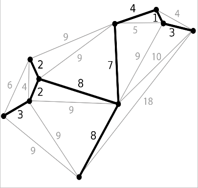
Using this method we know the lower bound of the solution – as the shortest distance must be above this. We can also use this to estimate how far we are from the perfect route. If the minimal spanning tree distance is 100 miles and a route we have found is 110 miles, we know that we are at most 10% from the perfect route – so we can calculate how close we are. Today’s algorithms can find routes which are less than 0.05% of the perfect route, no matter how many destinations in the list. This is a very good degree of certainty and vastly improves the time and space used to find it.

Continuous Relaxation

The travelling salesman problem is what is know as a ‘discrete optimisation problem.’ This is because the optimal route can only take discrete values: city A then city B then city C etc… A different approach is to relax the problem into a ‘continuous optimisation problem.’ This means to assign decimal values or fractions to each path and destination based on mathematical functions which evaluate them. This obviously would not give you a final answer, since you cannot go to two places at once and split the travelling salesman say one third to city A and two thirds to city B. However, what this approach can do is give you a better idea of the relationships between certain locations which can help to determine better routes. You could use the decimals values to create a strategy e.g. go with the biggest/smallest decimal every time.

Langranian Relaxation

A Langranian approach redefines the rules of the problem. It takes the constraints of a problem and converts them into cost functions. An algorithm can break these rules, however it will affect its overall score. Again this freedom given to an algorithm can help it to make much more progress in finding effective strategies. Even if you cannot use one of the routes because it breaks the constraints, you can identify patterns which otherwise would not have been seen. If these rules are not compulsory, you can actually find very good results in a very short amount of time. This idea is used in sports fixtures. Often there are rules set by the sport’s association, television broadcasters and key dates which control when certain games can be scheduled. However taking a Langranian approach to give the schedulers more freedom can prove vital in finding a much better fixture list. Letting some people down is much better than creating a poor list that the follows the rules.

The Langranian Wedding

In between studying for her chemical engineering PhD and planning her wedding, Meghan Bellows noticed a remarkable similarity between her work. At Princeton University, Bellows was studying how the location of amino acids in a protein chain correlate to a molecule’s particular characteristics. However at home she was trying to find the best seating arrangement for her 107 guests at her wedding with limited success. It then struck her that the two problems were the same! The amino acids were the people, the binding energies were the relationships and the molecules’ neighbour interactions were the guests’ neighbouring interactions. She used her knowledge in chemical engineering to recreate the problem. She worked though the guests, giving them scores between their relationships e.g. a couple would get a 10 whilst two strangers would get a 0. She then created a program which would attempt to find the optimum seating arrangement, the goal being to maximize the relationships score. However with the 11 tables seating 10 people each and the 107 guests, there were 11¹⁰⁷ possible seating arrangements. Even for her lab’s supercomputers this was too much computation. Here Langranian relaxation came to help. Bellows still allowed the computer program to run 36 hours and despite only getting a small fraction of the way through, it had yielded some helpful results. Among the best strategies so far, Bellows noticed relationships she had never even thought of and even ways to work around the constraints she had made. For example, she realised her parents did not necessarily need to sit on the family table which was already too full. Instead they could sit with old friends they had not seen for a while. This reversed Langranian approach (removing constraints after) helped Bellows to create a massively successful seating arrangement which her guests commended.

Hill Climbing

When we are faced with such discrete optimisation problems, another strategy can be extremely effective; randomness. When a problem has many permutations which could lead to the optimal solution, you can judge the quality of each permutation. Some permutations will be better than others and if you were to graph these solution qualities, you would end up with an ‘error landscape’ which compares the permutations visually:

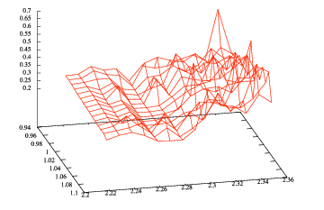
This shows that using certain calculus techniques, we can search for local maxima or minima to return the best solutions. Changing certain values will either push you up or down the error landscape. If your goal is to get the highest score (a maxima) you only want to commit to factors which increase your score. This is where randomness comes in. The process decides a random factor to change by a random value and if it helps you to get closer to your goal, you stick with it, otherwise you do the reverse. This is the process of hill climbing. As soon as you get to a point where changing any one factor decreases the permutation quality, you have not reached the best answer (the global maxima) but you have reached a local maxima, a good answer. Unfortunately this could be quite far from the global maxima and act as a ‘trap’ so there is another element you must add to the strategy. This element is called ‘jitter.’ If things are slowing down, perform some more random changes to random factors, even if it decreases your permutation quality. Then return to the hill climbing strategy. This technique can help you to get out of local maxima traps and be on your way towards the local maxima which is the best permutation. This is what a back propagation algorithm uses in a neural network to minimize the cost function.

Overfitting

When creating a model to predict data, it is important that the model is not too specific to that data. If this happens, the model will only work with the data used to create the model. It will not depict the relationship you want/need to see and when you go to use the model to find unknowns, you will get incorrect responses. When charting two factors, x and y, you may end up with a parabolic curve. You can add more factors to the chart e.g. x2, x3, x4… and so on. This will add more inflections to chart and the data points will fit the curve more accurately as you can see below on the blue line:

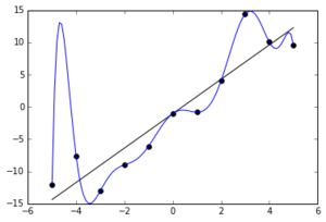
The model then becomes poor at predicting future values. In the example above, the x and y values follow a linear relationship (the black line) but the overfitted model will not show this and therefore is not suitable. This is a big problem in computer science, especially in machine learning processes which keep improving themselves. These models need to be broader. This is overfitting.

Overfitting Our Lives

Computers are not the only culprit of overfitting. Humans also overfit in many aspects of life. In early stages of human life, taste was a tool to help humans to identify what food is good for us and what food is bad for us. Ironically, we have optimised our taste bud model to know exactly what foods taste the best and this tends to be very salty or very sugary food which is now unhealthy for us. Overfitting is also evident in sport. Fencing was a sport derived from sword fighting, with the original goal of how to defend yourself. Today, however, professional fencers have mastered the art of flicking a fencing sword to bend it into the opponent which would not have been possible in traditional sword fights. This reward focused overfitting has caused the sport to lose sight of its original intentions. A similar process happens in the world of business where employees are rewarded on a scale of measurement. For example a lawyer who is rewarded in correlation to the number of cases they win might only pick easy cases over more urgent ones. They are not necessarily doing the wrong thing, rather they are doing the right thing so much it can actually harm the company. Overfitting is particularly evident in police training. Officers will sometimes empty their pockets after a shoot out to find the brass shells of the bullets in their pockets. They had actually put themselves in danger to pick up the shells during the shoot out, since this is good etiquette in the training centre. This is often referred to as ‘training scars.’ A more extreme example was when a police officer actually returned the gun to an assailant after he had disarmed them – just as he had done with his trainers in practice. This is a further example of people being so optimised to a process (like training drills) that some small unintentional parts become routine. Their model has become optimised to the point that it is less suitable for the real world scenarios.

Countering Overfitting

The way to fight overfitting is to penalize complexity. To do this we add constraints to our algorithms. This means that more complex models need to do a better job of justifying why the model needs to be more complex. Computer scientists refer to this process as Regularisation. One example constraint is a ‘Lasso’ algorithm invented in 1996 by biostatistician Robert Tibshirani. The Lasso uses weights which controls the contribution of a factor to an overall sum. This means certain factors will have to be significantly large or small to have an effect on the overall function and change the model. This is very commonly used in artificial neural networks which value certain inputs more for certain areas of the network. For example a facial recognition neural network might have a greater weight for pixels central to the image when trying to recognise the face’s nose. A bias is another method which neural networks use to regularise the feed forward algorithm to ensure that the correct inputs have the correct impact on the network.

Conclusion

Optimisation and overfitting are two massively important problems to both computer science and our world and it was very interesting to learn more about them. I particularly enjoyed learning about how our computer science approach to such problems can help us to solve real world problems of a similar type. I like the correlation between optimisation and overfitting. You want to optimise an algorithm just the right amount. Too little and program will yield poor results. Too much and the program will only return good results for the data used to form it – overfitting. I look forward to learning more about such problems and I am excited to have a go at tackling them.

Bibliography

• All research for this project came from the book “Algorithms to Live By” by Brian Christian and Tom Griffiths. I found these two topics particularly interesting and wanted to cover them in more detail in a research project.